David Firth published a paper in 1993 on maximum likelihood estimation and the reduction of bias when using this approach. The research in this area appears to provide benefit for logistic regression in small data sets where there is complete of quasi separation. This approach has been implemented for Generalized Linear Models in the brglm package.
Fast Tube by Casper
The help file for the brglm package provides the following words/justification about the methodology:
For estimation in binomial-response GLMs, the bias-reduction method is an improvement over traditional maximum likelihood because: • the bias-reduced estimator is second-order unbiased and has smaller variance than the maximum likelihood estimator and • the resultant estimates and their corresponding standard errors are always finite while the maximum likelihood estimates can be infinite (in situations where complete or quasi separation occurs). |
The original reference for this work is Firth, D. (1993). Bias reduction of maximum likelihood estimates. Biometrika 80, 27–38.
We will consider two data sets to compare the parameter estimates for a simple logistic regression model with one explanatory variable. The first example is one where we would expect a similar answer and the second is based on separation and illustrates the differences between the parameter estimates for the glm and brglm functions in R.
The first data set is shown below:
> ex1 = data.frame(
+ X = c(10, 10, 10, 20, 20, 20, 30, 30, 30, 40, 40, 40),
+ Y = c(0, 0, 0, 1, 0, 0, 1, 0, 1, 1, 1, 1)
+ )
> xtabs( ~ X + Y, data = ex1)
    Y
X    0 1
  10 3 0
  20 2 1
  30 1 2
40 0 3 |
The cross-tabulation shows that for the middle two values for the explanatory variable (X) we have a probability of 0.33 and 0.67. The logistic regression model fitted by glm to this data:
> m1a = glm(Y ~ X, data = ex1, family = binomial)
> summary(m1a)

Call:
glm(formula = Y ~ X, family = binomial, data = ex1)

Deviance Residuals:
    Min       1Q   Median       3Q      Max
-1.6877  -0.3734   0.0000   0.3734   1.6877

Coefficients:
            Estimate Std. Error z value Pr(>|z|)
(Intercept)  -5.7440     3.1622  -1.816   0.0693 .
X             0.2298     0.1214   1.892   0.0585 .
---
Signif. codes:  0 ‘***’ 0.001 ‘**’ 0.01 ‘*’ 0.05 ‘.’ 0.1 ‘ ’ 1

(Dispersion parameter for binomial family taken to be 1)

    Null deviance: 16.636  on 11  degrees of freedom
Residual deviance:  8.276  on 10  degrees of freedom
AIC: 12.276

Number of Fisher Scoring iterations: 5 |
The biased reduced version of this model:
> require(brglm)
Loading required package: brglm
Loading required package: profileModel

> m1b = brglm(Y ~ X, data = ex1, family = binomial)
> summary(m1b)

Call:
brglm(formula = Y ~ X, family = binomial, data = ex1)


Coefficients:
            Estimate Std. Error z value Pr(>|z|)
(Intercept) -3.90201    2.23945  -1.742   0.0814 .
X            0.15608    0.08439   1.849   0.0644 .
---
Signif. codes:  0 ‘***’ 0.001 ‘**’ 0.01 ‘*’ 0.05 ‘.’ 0.1 ‘ ’ 1

(Dispersion parameter for binomial family taken to be 1)

    Null deviance: 12.2045  on 11  degrees of freedom
Residual deviance:  8.7505  on 10  degrees of freedom
Penalized deviance: 3.23312
AIC: 12.751 |
In both cases the model has similar slope estimates for the explanatory variable and finite standard errors.
The next block of codes creates a graph to compare the two model fitting procedures.
> ex1a = data.frame( + Model = "GLM", + X = seq(0, 50), + Y = predict(m1a, newdata = data.frame(X = seq(0, 50)), type = "response") + ) > ex1b = data.frame( + Model = "BRGLM", + X = seq(0, 50), + Y = predict(m1b, newdata = data.frame(X = seq(0, 50)), type = "response") + ) > ex1c = rbind(ex1a, ex1b) > require(ggplot2) Loading required package: ggplot2 > ggplot(ex1c, aes(X, Y, colour = Model)) + geom_line() |
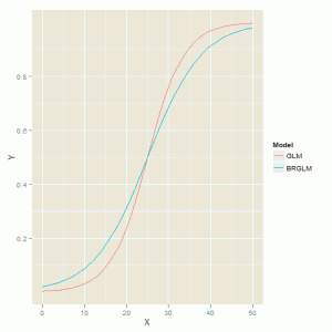
The fitted model curves are shown in the figure below which highlights the difference in slopes where the biased reduced model has a shallow curve compared to the model fitted by the glm function.
The second example is one where there is separation in the data – the probabilities of success are either 0 or 1 at all four values of the explanatory variable.
> ex2 = data.frame(
+ X = c(10, 10, 10, 20, 20, 20, 30, 30, 30, 40, 40, 40),
+ Y = c(0, 0, 0, 0, 0, 0, 1, 1, 1, 1, 1, 1)
+ )
>
> xtabs( ~ X + Y, data = ex2)
    Y
X    0 1
  10 3 0
  20 3 0
  30 0 3
40 0 3 |
The glm function struggles to produce a sensible fit to the data and the standard errors for the model parameters are very large.
> m2a = glm(Y ~ X, data = ex2, family = binomial)
Warning message:
glm.fit: fitted probabilities numerically 0 or 1 occurred
> summary(m2a)

Call:
glm(formula = Y ~ X, family = binomial, data = ex2)

Deviance Residuals:
       Min          1Q      Median          3Q         Max
-6.326e-06  -1.597e-06   0.000e+00   1.597e-06   6.326e-06

Coefficients:
              Estimate Std. Error z value Pr(>|z|)
(Intercept)   -123.174 282264.199       0        1
X                4.927  11071.305       0        1

(Dispersion parameter for binomial family taken to be 1)

    Null deviance: 1.6636e+01  on 11  degrees of freedom
Residual deviance: 2.4010e-10  on 10  degrees of freedom
AIC: 4

Number of Fisher Scoring iterations: 25 |
The bias reduced version provides finite estimate of the model parameters:
> m2b = brglm(Y ~ X, data = ex2, family = binomial)
> summary(m2b)

Call:
brglm(formula = Y ~ X, family = binomial, data = ex2)


Coefficients:
            Estimate Std. Error z value Pr(>|z|)
(Intercept)  -8.2336     4.7028  -1.751    0.080 .
X             0.3293     0.1831   1.799    0.072 .
---
Signif. codes:  0 ‘***’ 0.001 ‘**’ 0.01 ‘*’ 0.05 ‘.’ 0.1 ‘ ’ 1

(Dispersion parameter for binomial family taken to be 1)

    Null deviance: 12.55  on 11  degrees of freedom
Residual deviance:  2.20  on 10  degrees of freedom
Penalized deviance: -1.03921
AIC: 6.2 |
In a similar fashion we can compare the fitted model in both cases:
> ex2a = data.frame( + Model = "GLM", + X = seq(0, 50), + Y = predict(m2a, newdata = data.frame(X = seq(0, 50)), type = "response") + ) > ex2b = data.frame( + Model = "BRGLM", + X = seq(0, 50), + Y = predict(m2b, newdata = data.frame(X = seq(0, 50)), type = "response") + ) > ex2c = rbind(ex2a, ex2b) ggplot(ex2c, aes(X, Y, colour = Model)) + geom_line() |
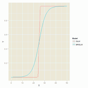
The figure below is the comparison of the two fitting methods and we can see that the glm function produces a model that is not far off a step function which is unsatisfactory description of the data.
Other useful resources are provided on the Supplementary Material page.


Hallo there,
I tried to reproduce the your code just to see whether it would work,
but the third part of it didn’t. Have you got any idea as to how to compare the fitted model in both cases?
Thanks a lot.
AA
m1a = glm(hollyday~ income, data = household, family = binomial)
summary(m1a)
confint(m1a)
Call:
glm(formula = hollyday ~ income, family = binomial, data = household)
Deviance Residuals:
Min 1Q Median 3Q Max
-2.2418 0.4111 0.4111 0.4111 0.8544
Coefficients:
Estimate Std. Error z value Pr(>|z|)
(Intercept) 0.8199 0.1973 4.155 3.25e-05 ***
income[T.low] 1.6085 0.2523 6.375 1.83e-10 ***
—
Signif. codes: 0 ‘***’ 0.001 ‘**’ 0.01 ‘*’ 0.05 ‘.’ 0.1 ‘ ‘ 1
(Dispersion parameter for binomial family taken to be 1)
Null deviance: 492.51 on 663 degrees of freedom
Residual deviance: 454.47 on 662 degrees of freedom
AIC: 458.47
The biased reduced version of this model:
require(brglm)
m1b = brglm(Holiday~ income, data = household, family = binomial)
summary(m1b)
Call:
brglm(formula = Holiday ~ income, family = binomial,
data = household)
Coefficients:
Estimate Std. Error z value Pr(>|z|)
(Intercept) 0.8161 0.1394 5.854 4.8e-09 ***
income[T.low] 1.6071 0.1782 9.019 < 2e-16 ***
—
Signif. codes: 0 '***' 0.001 '**' 0.01 '*' 0.05 '.' 0.1 ' ' 1
(Dispersion parameter for binomial family taken to be 1)
Null deviance: 973.62 on 1327 degrees of freedom
Residual deviance: 908.94 on 1326 degrees of freedom
Penalized deviance: 900.5998
AIC: 912.94
Hi,
Could you explain how the last part of the code failed to run?
Did you get any error messages?
Did the graph plot but without the lines?
For your example the explanatory variable income is categorical unlike my example where it is continuous so a similar graph does not make sense I think.
Thanks
R
Hi,
Is there a version of the video with better sound quality? I was unable to hear what was being said.
I would probably would need to record the video again which would be better than leaving an incomprehensible video up! Thank you for flagging this up.