The Generalized Additive Models for Location, Scale and Shape (GAMLSS) is a recent development which provides a framework with access to a large set of distributions and the ability to model all of the parameters of these distributions as functions of the explanatory variables within a data set.
Fast Tube by Casper
We can take a look at the gamlss function, which is the workhorse of the package, with a simulated data set using the random number generator for the Normal Distribution. We create a simple example where there are three groups, each with twenty observations, where the mean and standard deviation are different for each group.
d1.N = 20

d1 = data.frame(
    Group = c(
        rep("A", d1.N),
        rep("B", d1.N),
        rep("C", d1.N)
    ),
    Response = c(
        rnorm(d1.N, mean = 15, sd = 3),
        rnorm(d1.N, mean = 12, sd = 6),
        rnorm(d1.N, mean = 19, sd = 8)
    )
) |
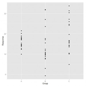
An example of data generated using the above code is shown in the following graph and we can see the differences in the variability of each group.
The gamlss model is fitted with a specification of the distribution (NO) and a formula describing how the mean and standard deviation of the Normal distribution vary based on the Group.
d1.gamlss1 = gamlss(
    Response ~ Group,
    sigma.formula = ~ Group,
    data = d1,
    family = NO
) |
We can get a summary of the fitted model:
> summary(d1.gamlss1)
*******************************************************************
Family:  c("NO", "Normal")

Call:  gamlss(formula = Response ~ Group, sigma.formula = ~Group, family = NO,
    data = d1)

Fitting method: RS()

-------------------------------------------------------------------
Mu link function:  identity
Mu Coefficients:
             Estimate  Std. Error  t value   Pr(>|t|)
(Intercept)    15.656      0.6214  25.1941  1.577e-31
GroupB         -1.525      2.0166  -0.7564  4.527e-01
GroupC          3.067      1.8598   1.6492  1.049e-01

-------------------------------------------------------------------
Sigma link function:  log
Sigma Coefficients:
             Estimate  Std. Error  t value   Pr(>|t|)
(Intercept)     1.022      0.1581    6.464  3.044e-08
GroupB          1.127      0.2236    5.041  5.534e-06
GroupC          1.037      0.2236    4.638  2.278e-05

-------------------------------------------------------------------
No. of observations in the fit:  60
Degrees of Freedom for the fit:  6
      Residual Deg. of Freedom:  54
                      at cycle:  2

Global Deviance:     379.4989
            AIC:     391.4989
            SBC:     404.065
******************************************************************* |
The coefficients in the summary table are used to generate the formula for estimating the mean and standard deviation. Note that the standard deviation is on the natural log scale so needs to be converted to the original scale, e.g. exp(1.022) for Group A.
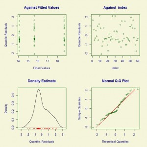
The standard set of diagnostic plots are generated via the plot function.
The plot is generally ok with a few observations that are not as expected.
This post is a very brief look at the GAMLSS framework which provides a lot additional functionality.


