The Generalized Linear Model (GLM) allows us to model responses with distributions other than the Normal distribution, which is one of the assumptions underlying linear regression as used in many cases. When data is counts of events (or items) then a discrete distribution is more appropriate is usually more appropriate than approximating with a continuous distribution, especially as our counts should be bounded below at zero. Negative counts do not make sense.
Fast Tube by Casper
To investigate using Poisson regression via the GLM framework consider a small data set on failure modes (here).
> failure.df = read.table("twomodes.dat", header = TRUE)
> failure.df
  Mode1 Mode2 Failures
1  33.3  25.3       15
2  52.2  14.4        9
3  64.7  32.5       14
4 137.0  20.5       24
5 125.9  97.6       27
6 116.3  53.6       27
7 131.7  56.6       23
8  85.0  87.3       18
9 91.9 47.8 22 |
The machinery is run in two modes and the objective of the analysis is to determine whether the number of failures depends on how long the machine is run in mode 1 or mode 2 and whether there is an interaction between the time in each mode to increases or decreases the number of failures.
The response for this set of data is the number of failures (count) so a Poisson regression model is considered.
> fmod1 = glm(Failures ~ Mode1 * Mode2, data = failure.df, family = poisson)
> summary(fmod1)

Call:
glm(formula = Failures ~ Mode1 * Mode2, family = poisson, data = failure.df)

Deviance Residuals:
       1         2         3         4         5         6         7         8         9
 0.91003  -1.15601  -0.28328  -0.10398   0.03526   0.84825  -0.49211  -0.57298   0.64821

Coefficients:
              Estimate Std. Error z value Pr(>|z|)
(Intercept)  2.105e+00  4.481e-01   4.698 2.63e-06 ***
Mode1        7.687e-03  4.285e-03   1.794   0.0729 .
Mode2        4.703e-03  1.163e-02   0.405   0.6858
Mode1:Mode2 -1.978e-05  1.037e-04  -0.191   0.8487
---
Signif. codes:  0 ‘***’ 0.001 ‘**’ 0.01 ‘*’ 0.05 ‘.’ 0.1 ‘ ’ 1

(Dispersion parameter for poisson family taken to be 1)

    Null deviance: 16.996  on 8  degrees of freedom
Residual deviance:  3.967  on 5  degrees of freedom
AIC: 55.024

Number of Fisher Scoring iterations: 4 |
The model output does not provide any support for an interaction between the number of time spent in the two different modes of operation. If we remove the interaction term and re-fit the model, using the update function, we get:
> fmod2 = update(fmod1, . ~ . - Mode1:Mode2)
> summary(fmod2)

Call:
glm(formula = Failures ~ Mode1 + Mode2, family = poisson, data = failure.df)

Deviance Residuals:
     Min        1Q    Median        3Q       Max
-1.21984  -0.44735  -0.05893   0.68351   0.87510

Coefficients:
            Estimate Std. Error z value Pr(>|z|)
(Intercept) 2.175168   0.255456   8.515  < 2e-16 ***
Mode1       0.007015   0.002429   2.888  0.00387 **
Mode2       0.002549   0.002835   0.899  0.36852
---
Signif. codes:  0 ‘***’ 0.001 ‘**’ 0.01 ‘*’ 0.05 ‘.’ 0.1 ‘ ’ 1

(Dispersion parameter for poisson family taken to be 1)

    Null deviance: 16.9964  on 8  degrees of freedom
Residual deviance:  4.0033  on 6  degrees of freedom
AIC: 53.06

Number of Fisher Scoring iterations: 4 |
This output suggests that the time of operation in mode 1 is important for determining the number of faults but the time of operation in mode 2 is not important. One last step gives us:
> fmod3 = update(fmod2, . ~ . - Mode2)
> summary(fmod3)

Call:
glm(formula = Failures ~ Mode1, family = poisson, data = failure.df)

Deviance Residuals:
     Min        1Q    Median        3Q       Max
-1.43194  -0.56958  -0.00745   0.66742   0.82231

Coefficients:
            Estimate Std. Error z value Pr(>|z|)
(Intercept) 2.237196   0.243053   9.205  < 2e-16 ***
Mode1       0.007705   0.002264   3.403 0.000667 ***
---
Signif. codes:  0 ‘***’ 0.001 ‘**’ 0.01 ‘*’ 0.05 ‘.’ 0.1 ‘ ’ 1

(Dispersion parameter for poisson family taken to be 1)

    Null deviance: 16.9964  on 8  degrees of freedom
Residual deviance:  4.8078  on 7  degrees of freedom
AIC: 51.865

Number of Fisher Scoring iterations: 4 |
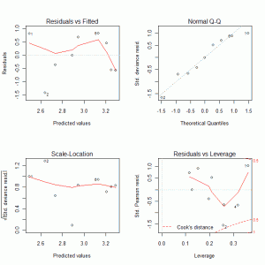
The diagnostic plots are shown below which do not indicate any major problems with the final model, especially given the small number of data points.
Other useful resources are provided on the Supplementary Material page.


I am using the Capture recapture technique to estimate population size and mortality of African jacanas (open population),16 capture missions were done over a period of 4 yrs.How best can i use R to achive my objective?
Hi Buleya,
Have you considered the package Rcapture? It appears to have some functionality that might be useful for your work.
Hope this helps,
Ralph