The simple linear regression model considers the relationship between two variables and in many cases more information will be available that can be used to extend the model. For example, there might be a categorical variable (sometimes known as a covariate) that can be used to divide the data set to fit a separate linear regression to each of the subsets. We will consider how to handle this extension using one of the data sets available within the R software package.
There is a set of data relating trunk circumference (in mm) to the age of Orange trees where data was recorded for five trees. This data is available in the data frame Orange and we make a copy of this data set so that we can remove the ordering that is recorded for the Tree identifier variable. We create a new factor after converting the old factor to a numeric string:
orange.df = Orange orange.df$Tree = factor(as.numeric(orange.df$Tree)) |
The purpose of this step is to set up the variable for use in the linear model. The simplest model assumes that the relationship between circumference and age is the same for all five trees and we fit this model as follows:
orange.mod1 = lm(circumference ~ age, data = orange.df) |
The summary of the fitted model is shown here:
> summary(orange.mod1)

Call:
lm(formula = circumference ~ age, data = orange.df)

Residuals:
      Min        1Q    Median        3Q       Max
-46.31030 -14.94610  -0.07649  19.69727  45.11146

Coefficients:
             Estimate Std. Error t value Pr(>|t|)
(Intercept) 17.399650   8.622660   2.018   0.0518 .
age          0.106770   0.008277  12.900 1.93e-14 ***
---
Signif. codes:  0 ‘***’ 0.001 ‘**’ 0.01 ‘*’ 0.05 ‘.’ 0.1 ‘ ’ 1

Residual standard error: 23.74 on 33 degrees of freedom
Multiple R-squared: 0.8345,     Adjusted R-squared: 0.8295
F-statistic: 166.4 on 1 and 33 DF, p-value: 1.931e-14 |
The test on the age parameter provides very strong evidence of an increase in circumference with age, as would be expected. The next stage is to consider how this model can be extended – one idea is to have a separate intercept for each of the five trees. This new model assumes that the increase in circumference is consistent between the trees but that the growth starts at different rates. We fit this model and get the summary as follows:
> orange.mod2 = lm(circumference ~ age + Tree, data = orange.df)
> summary(orange.mod2)

Call:
lm(formula = circumference ~ age + Tree, data = orange.df)

Residuals:
    Min      1Q  Median      3Q     Max
-30.505  -8.790   3.738   7.650  21.859

Coefficients:
             Estimate Std. Error t value Pr(>|t|)
(Intercept) -4.457493   7.572732  -0.589   0.5607
age          0.106770   0.005321  20.066  < 2e-16 ***
Tree2        5.571429   8.157252   0.683   0.5000
Tree3       17.142857   8.157252   2.102   0.0444 *
Tree4       41.285714   8.157252   5.061 2.14e-05 ***
Tree5       45.285714   8.157252   5.552 5.48e-06 ***
---
Signif. codes:  0 ‘***’ 0.001 ‘**’ 0.01 ‘*’ 0.05 ‘.’ 0.1 ‘ ’ 1

Residual standard error: 15.26 on 29 degrees of freedom
Multiple R-squared: 0.9399,     Adjusted R-squared: 0.9295
F-statistic: 90.7 on 5 and 29 DF, p-value: < 2.2e-16 |
The additional term is appended to the simple model using the + in the formula part of the call to lm. The first tree is used as the baseline to compare the other four trees against and the model summary shows that tree 2 is similar to tree 1 (no real need for a different offset) but that there is evidence that the offset for the other three trees is significantly larger than tree 1 (and tree 2). We can compare the two models using an F-test for nested models using the anova function:
> anova(orange.mod1, orange.mod2) Analysis of Variance Table Model 1: circumference ~ age Model 2: circumference ~ age + Tree Res.Df RSS Df Sum of Sq F Pr(>F) 1 33 18594.7 2 29 6753.9 4 11841 12.711 4.289e-06 *** --- Signif. codes: 0 ‘***’ 0.001 ‘**’ 0.01 ‘*’ 0.05 ‘.’ 0.1 ‘ ’ 1 |
Here there are four degrees of freedom used up by the more complicated model (four parameters for the different trees) and the test comparing the two models is highly significant. There is very strong evidence of a difference in starting circumference (for the data that was collected) between the trees.
We can extended this model further by allowing the rate of increase in circumference to vary between the five trees. This additional term can be included in the linear model as an interaction term, assuming that tree 1 is the baseline. An interaction term is included in the model formula with a : between the name of two variables. For the Orange tree data the new model is fitted thus:
> orange.mod3 = lm(circumference ~ age + Tree + age:Tree, data = orange.df)
> summary(orange.mod3)

Call:
lm(formula = circumference ~ age + Tree + age:Tree, data = orange.df)

Residuals:
    Min      1Q  Median      3Q     Max
-18.061  -6.639  -1.482   8.069  16.649

Coefficients:
              Estimate Std. Error t value Pr(>|t|)
(Intercept)  1.920e+01  8.458e+00   2.270  0.03206 *
age          8.111e-02  8.119e-03   9.991 3.27e-10 ***
Tree2        5.234e+00  1.196e+01   0.438  0.66544
Tree3       -1.045e+01  1.196e+01  -0.873  0.39086
Tree4        7.574e-01  1.196e+01   0.063  0.95002
Tree5       -4.566e+00  1.196e+01  -0.382  0.70590
age:Tree2    3.656e-04  1.148e-02   0.032  0.97485
age:Tree3    2.992e-02  1.148e-02   2.606  0.01523 *
age:Tree4    4.395e-02  1.148e-02   3.828  0.00077 ***
age:Tree5    5.406e-02  1.148e-02   4.708 7.93e-05 ***
---
Signif. codes:  0 ‘***’ 0.001 ‘**’ 0.01 ‘*’ 0.05 ‘.’ 0.1 ‘ ’ 1

Residual standard error: 10.41 on 25 degrees of freedom
Multiple R-squared: 0.9759,     Adjusted R-squared: 0.9672
F-statistic: 112.4 on 9 and 25 DF, p-value: < 2.2e-16 |
Interesting we see that there is strong evidence of a difference in the rate of change in circumference for the five trees. The previously observed difference in intercepts is now longer as strong but this parameter is kept in the model – there are plenty of books/websites that discuss this marginality restrictin on statistical models. The fitted model described above can be created using lattice graphics with a custom panel function making use of available panel functions for fitting and drawing a linear regression line for each panel of a Trellis display. The function call is shown below:
xyplot(circumference ~ age | Tree, data = orange.df,
  panel = function(x, y, ...)
  {
    panel.xyplot(x, y, ...)
    panel.lmline(x, y, ...)
  }
) |
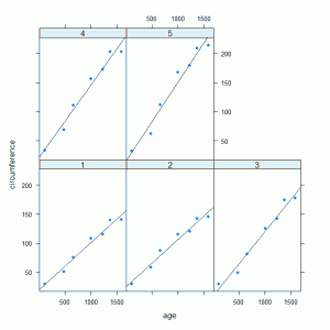
The panel.xyplot and panel.lmline functions are part of the lattice package along with many other panel functions and can be built up to create a display that differs from the standard. The graph that is produced:
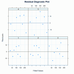
This graph clearly shows the different relationships between circumference and age for the five trees. The residuals from the model can be plotted against fitted values, divided by tree, to investigate the model assumptions:
xyplot(resid(orange.mod3) ~ fitted(orange.mod3) | orange.df$Tree,
  xlab = "Fitted Values",
  ylab = "Residuals",
  main = "Residual Diagnostic Plot",
  panel = function(x, y, ...)
  {
    panel.grid(h = -1, v = -1)
    panel.abline(h = 0)
    panel.xyplot(x, y, ...)
  }
) |
The residual diagnostic plot is:
There are no obvious problematic patterns in this graph so we conclude that this model is a reasonable representation of the relationship between circumference and age.
Additional: The analysis of variance table comparing the second and third models shows an improvement by moving to the more complicated model with different slopes:
> anova(orange.mod2, orange.mod3) Analysis of Variance Table Model 1: circumference ~ age + Tree Model 2: circumference ~ age + Tree + age:Tree Res.Df RSS Df Sum of Sq F Pr(>F) 1 29 6753.9 2 25 2711.0 4 4042.9 9.3206 9.402e-05 *** --- Signif. codes: 0 ‘***’ 0.001 ‘**’ 0.01 ‘*’ 0.05 ‘.’ 0.1 ‘ ’ 1 |


Can we see the anova(orange.mod2, orange.mod3) results? Are the separate slopes fitting better than the separate intercepts?
Thanks for pointing out that oversight on my behalf – will add to the end of the post.
You said, “There are no obvious problematic patterns” in the residuals. However, there is some structure that is quite obvious (once you see it the first time). Notice that at time point 2 the residuals are negative (for all trees) and at time point 6 the residuals are positive (for all trees). Clearly, there is structure that is not completely modeled by the linear fit. Pinheiro & Bates in the MEMSS book fit a logistic function to this data. The ASREML-R manual shows how to fit a spline to this data. Both methods provide better fits than the linear model.
On reflection, in addition to the negative residuals at the second time point, there are also negative residuals for the last time point in all trees. This provides more support to the use of the logistic growth model as a more appropriate model for this data due to being bounded below and above. The non-linear model has interpretable parameters which is another benefit. As you say, the initially non obvious patterns stand out once they have been pointed out!
Thanks. your simple language cleared up some questions that I had regarding factors in lm and interaction variables
Another way to specify the interaction term is:
> orange.mod3 = lm(circumference ~ (age * Tree)^2 , data = orange.df)
> summary(orange.mod3)
In models with more complicated relations this can be a time-saver.
“there are plenty of books/websites that discuss this marginality restrictin on statistical models”
Could you please give some hints on what you mean?
I’m not sure that this is pertinent in this case, but a graph of all Residuals vs Fitted shows some non-linear relationship. Also, the QQ plot doesn’t look very normal.
oldpar <- par(oma=c(0,0,3,0), mfrow=c(2,2))
plot(orange.mod3)
par(oldpar)
The marginality restriction is concerned with situations where an interaction term is significant but one (or more) of the variables that make up the interaction are not significant. In these situations the convention is to include all of the variables. One way people think about this is to consider the quadratic equation a + bx + cx^2 and in this situation we would have b not being significant but c being significant. If we excluded the b from this function to leave a + cx^2 then we would have less flexibility as this function is centred around x = 0 which may not be desirable.
Hope this helps.
Compared to other statistics software systems the model formula approach in S is very flexible especially when used in conjunction with the update function when moving through a range of possible models when there are a large number of variables of potential interest.
On a side note orange.mod3 = lm(circumference ~ age * Tree , data = orange.df) will also fit the same model. I think this is because the ^2 requests all terms involving pairs of the variables which because we only have two variables includes the two-way interaction. If you have more variables and were only interested in the two-way interactions and nothing higher than that then your code does the job nicely!
Yes, this gives me an idea about the marginality restriction. Also, I wasn’t aware of the update() fun. Looks interesting. Thanks