One of the most frequent used techniques in statistics is linear regression where we investigate the potential relationship between a variable of interest (often called the response variable but there are many other names in use) and a set of one of more variables (known as the independent variables or some other term). Unsurprisingly there are flexible facilities in R for fitting a range of linear models from the simple case of a single variable to more complex relationships.
In this post we will consider the case of simple linear regression with one response variable and a single independent variable. For this example we will use some data from the book Mathematical Statistics with Applications by Mendenhall, Wackerly and Scheaffer (Fourth Edition – Duxbury 1990). This data is for a study in central Florida where 15 alligators were captured and two measurements were made on each of the alligators. The weight (in pounds) was recorded with the snout vent length (in inches – this is the distance between the back of the head to the end of the nose).
The purpose of using this data is to determine whether there is a relationship, described by a simple linear regression model, between the weight and snout vent length. The authors analysed the data on the log scale (natural logarithms) and we will follow their approach for consistency. We first create a data frame for this study:
alligator = data.frame(
  lnLength = c(3.87, 3.61, 4.33, 3.43, 3.81, 3.83, 3.46, 3.76,
    3.50, 3.58, 4.19, 3.78, 3.71, 3.73, 3.78),
  lnWeight = c(4.87, 3.93, 6.46, 3.33, 4.38, 4.70, 3.50, 4.50,
    3.58, 3.64, 5.90, 4.43, 4.38, 4.42, 4.25)
) |
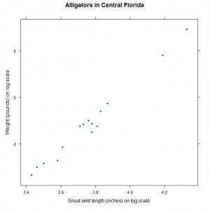
As with most analysis the first step is to perform some exploratory data analysis to get a visual impression of whether there is a relationship between weight and snout vent length and what form it is likely to take. We create a scatter plot of the data as follows:
xyplot(lnWeight ~ lnLength, data = alligator, xlab = "Snout vent length (inches) on log scale", ylab = "Weight (pounds) on log scale", main = "Alligators in Central Florida" ) |
The scatter plot is shown here:
The graph suggests that weight (on the log scale) increases linearly with snout vent length (again on the log scale) so we will fit a simple linear regression model to the data and save the fitted model to an object for further analysis:
alli.mod1 = lm(lnWeight ~ lnLength, data = alligator) |
The function lm fits a linear model to data are we specify the model using a formula where the response variable is on the left hand side separated by a ~ from the explanatory variables. The formula provides a flexible way to specify various different functional forms for the relationship. The data argument is used to tell R where to look for the variables used in the formula.
Now that the model is saved as an object we can use some of the general purpose functions for extracting information from this object about the linear model, e.g. the parameters or residuals. The big plus with R is that there are functions defined for different types of model, using the same name such as summary, and the system works out what function we intended to use based on the type of object saved. To create a summary of the fitted model:
> summary(alli.mod1)

Call:
lm(formula = lnWeight ~ lnLength, data = alligator)

Residuals:
     Min       1Q   Median       3Q      Max
-0.24348 -0.03186  0.03740  0.07727  0.12669

Coefficients:
            Estimate Std. Error t value Pr(>|t|)
(Intercept)  -8.4761     0.5007  -16.93 3.08e-10 ***
lnLength      3.4311     0.1330   25.80 1.49e-12 ***
---
Signif. codes:  0 ‘***’ 0.001 ‘**’ 0.01 ‘*’ 0.05 ‘.’ 0.1 ‘ ’ 1

Residual standard error: 0.1229 on 13 degrees of freedom
Multiple R-squared: 0.9808,     Adjusted R-squared: 0.9794
F-statistic: 665.8 on 1 and 13 DF, p-value: 1.495e-12 |
We get a lot of useful information here without being too overwhelmed by pages of output.
The estimates for the model intercept is -8.4761 and the coefficient measuring the slope of the relationship with snout vent length is 3.4311 and information about standard errors of these estimates is also provided in the Coefficients table. We see that the test of significance of the model coefficients is also summarised in that table so we can see that there is strong evidence that the coefficient is significantly different to zero – as the snout vent length increases so does the weight.
Rather than stopping here we perform some investigations using residual diagnostics to determine whether the various assumptions that underpin linear regression are reasonable for our data or if there is evidence to suggest that additional variables are required in the model or some other alterations to identify a better description of the variables that determine how weight changes.
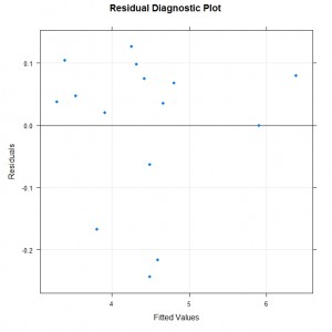
A plot of the residuals against fitted values is used to determine whether there are any systematic patterns, such as over estimation for most of the large values or increasing spread as the model fitted values increase. To create this plot we could use the following code:
xyplot(resid(alli.mod1) ~ fitted(alli.mod1),
  xlab = "Fitted Values",
  ylab = "Residuals",
  main = "Residual Diagnostic Plot",
  panel = function(x, y, ...)
  {
    panel.grid(h = -1, v = -1)
    panel.abline(h = 0)
    panel.xyplot(x, y, ...)
  }
) |
We create our own custom panel function using the buliding blocks provided by the lattice package. We start by creating a set of grid lines as the base layer and the h=-1 and v=-1 tell lattice to align these with the labels on the axes. We then create a solid horizontal line to help distinguish between positive and negative residuals. Finally we get the points plotted on the top layer.
The residual diagnostic plot is shown below:
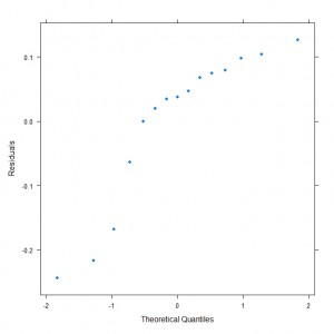
The plot is probably ok but there are more cases of positive residuals and when we consider a normal probability plot we see that there are some deficiencies with the model:
qqmath( ~ resid(alli.mod1), xlab = "Theoretical Quantiles", ylab = "Residuals" ) |
The function resid extracts the model residuals from the fitted model object. The plot is shown here:
We would hope that this plot showed something approaching a straight line to support the model assumption about the distribution of the residuals. This and the other plots suggest that further tweaking to the model is required to improve the model or a decision would need to be made about whether to report the model as is with some caveats about its usage. I am interested in the thoughts/comments/suggestions from how other people would proceed when faced with this situation – feel free to add in the comments.
Related posts:
- Manual variable selection with the dropterm function.
- The update function for simplifying model selection.
- Including factors in a regression model via analysis of covariance.


